


Intro
MNIST Image Classification with Keras

1. Setup
import tensorflow as tf
import tensorflow_datasets as tfds
from matplotlib import pyplot as plt
import numpy as np
2. Load the MNIST Dataset
- MNIST dataset: 28×28 grayscale images, 60,000 training samples, 10,000 testing samples
- Pixel values range from 0 to 255
- Load data with tf.keras.datasets.mnist.load_data
# Tuples of uint8 NumPy arrays
(x_train, y_train), (x_test, y_test) = tf.keras.datasets.mnist.load_data()

print("Training set:", x_train.shape, y_train.shape)
print("Test set:", x_test.shape, y_test.shape)
3. Visualize Sample Images
print(f"dtype: {x_train[0].dtype}, shape: {x_train[0].shape}")
print(x_train[0])
plt.imshow(x_train[0], cmap='gray')
Image structure (See Image Representation)
dtype: uint8, shape: (28, 28)
[[  0   0   0   0   0   0   0   0   0   0   0   0   0   0   0   0   0   0
    0   0   0   0   0   0   0   0   0   0]
 [  0   0   0   0   0   0   0   0   0   0   0   0   0   0   0   0   0   0
    0   0   0   0   0   0   0   0   0   0]
 [  0   0   0   0   0   0   0   0   0   0   0   0   0   0   0   0   0   0
    0   0   0   0   0   0   0   0   0   0]
 [  0   0   0   0   0   0   0   0   0   0   0   0   0   0   0   0   0   0
    0   0   0   0   0   0   0   0   0   0]
 [  0   0   0   0   0   0   0   0   0   0   0   0   0   0   0   0   0   0
    0   0   0   0   0   0   0   0   0   0]
 [  0   0   0   0   0   0   0   0   0   0   0   0   3  18  18  18 126 136
  175  26 166 255 247 127   0   0   0   0]
 [  0   0   0   0   0   0   0   0  30  36  94 154 170 253 253 253 253 253
  225 172 253 242 195  64   0   0   0   0]
 [  0   0   0   0   0   0   0  49 238 253 253 253 253 253 253 253 253 251
   93  82  82  56  39   0   0   0   0   0]
 [  0   0   0   0   0   0   0  18 219 253 253 253 253 253 198 182 247 241
    0   0   0   0   0   0   0   0   0   0]
 [  0   0   0   0   0   0   0   0  80 156 107 253 253 205  11   0  43 154
    0   0   0   0   0   0   0   0   0   0]
 [  0   0   0   0   0   0   0   0   0  14   1 154 253  90   0   0   0   0
    0   0   0   0   0   0   0   0   0   0]
 [  0   0   0   0   0   0   0   0   0   0   0 139 253 190   2   0   0   0
    0   0   0   0   0   0   0   0   0   0]
 [  0   0   0   0   0   0   0   0   0   0   0  11 190 253  70   0   0   0
    0   0   0   0   0   0   0   0   0   0]
 [  0   0   0   0   0   0   0   0   0   0   0   0  35 241 225 160 108   1
    0   0   0   0   0   0   0   0   0   0]
 [  0   0   0   0   0   0   0   0   0   0   0   0   0  81 240 253 253 119
   25   0   0   0   0   0   0   0   0   0]
 [  0   0   0   0   0   0   0   0   0   0   0   0   0   0  45 186 253 253
  150  27   0   0   0   0   0   0   0   0]
 [  0   0   0   0   0   0   0   0   0   0   0   0   0   0   0  16  93 252
  253 187   0   0   0   0   0   0   0   0]
 [  0   0   0   0   0   0   0   0   0   0   0   0   0   0   0   0   0 249
  253 249  64   0   0   0   0   0   0   0]
 [  0   0   0   0   0   0   0   0   0   0   0   0   0   0  46 130 183 253
  253 207   2   0   0   0   0   0   0   0]
 [  0   0   0   0   0   0   0   0   0   0   0   0  39 148 229 253 253 253
  250 182   0   0   0   0   0   0   0   0]
 [  0   0   0   0   0   0   0   0   0   0  24 114 221 253 253 253 253 201
   78   0   0   0   0   0   0   0   0   0]
 [  0   0   0   0   0   0   0   0  23  66 213 253 253 253 253 198  81   2
    0   0   0   0   0   0   0   0   0   0]
 [  0   0   0   0   0   0  18 171 219 253 253 253 253 195  80   9   0   0
    0   0   0   0   0   0   0   0   0   0]
 [  0   0   0   0  55 172 226 253 253 253 253 244 133  11   0   0   0   0
    0   0   0   0   0   0   0   0   0   0]
 [  0   0   0   0 136 253 253 253 212 135 132  16   0   0   0   0   0   0
    0   0   0   0   0   0   0   0   0   0]
 [  0   0   0   0   0   0   0   0   0   0   0   0   0   0   0   0   0   0
    0   0   0   0   0   0   0   0   0   0]
 [  0   0   0   0   0   0   0   0   0   0   0   0   0   0   0   0   0   0
    0   0   0   0   0   0   0   0   0   0]
 [  0   0   0   0   0   0   0   0   0   0   0   0   0   0   0   0   0   0
    0   0   0   0   0   0   0   0   0   0]]
plt.figure(figsize=(6,6))
for i in range(9):
    plt.subplot(3, 3, i + 1)
    plt.imshow(x_train[i], cmap="gray")
    plt.title(f"Label: {y_train[i]}")
    plt.axis("off")
plt.tight_layout()
plt.show()
4. Preprocess the Data
Transform the dataset into a format suitable for the neural network
Flatten the images
Reshape each image into a flat vector: (28, 28) → (784,)

x_train = x_train.reshape(60000, 784)
x_test = x_test.reshape(10000, 784)
print("Training set:", x_train.shape, y_train.shape)
print("Test set:", x_test.shape, y_test.shape)
Training set: (60000, 784) (60000,)
Test set: (10000, 784) (10000,)
Normalize the pixel values
- X_train = X_train.astype(‘float32’): Convert the training images to float32 type.
- X_test = X_test.astype(‘float32’): Convert the test images to float32 type.
- X_train /= 255: Normalize the training images’ pixel values to the range [0, 1].
- X_test /= 255: Normalize the test images’ pixel values to the range [0, 1].
x_train = x_train.astype('float32') / 255 # uint8 → float32
x_test = x_test.astype('float32') / 255
# print(x_train[0])
One-hot encode labels
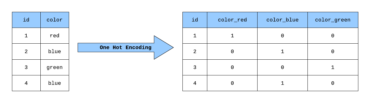
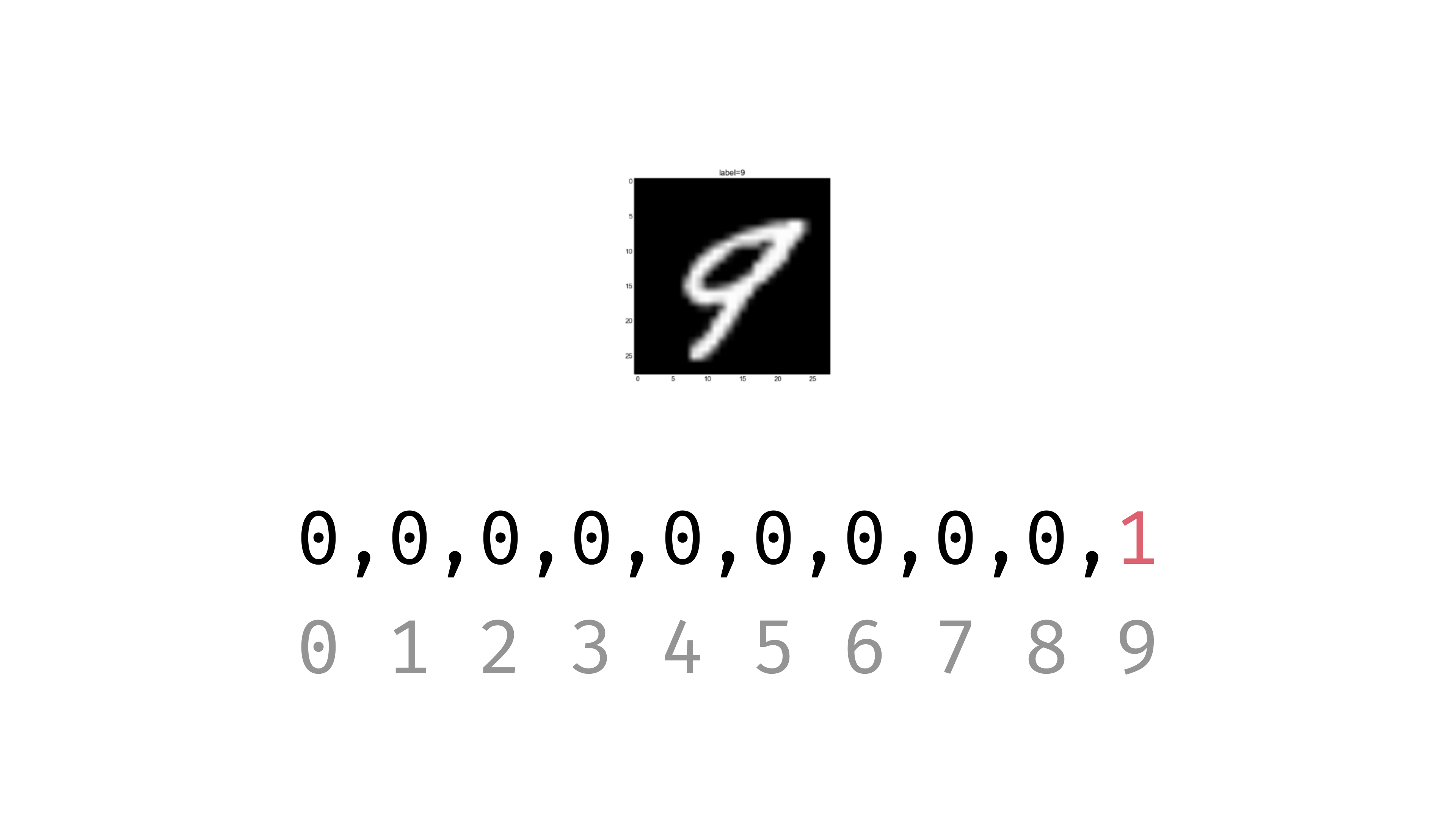
- Integer labels → One-hot vectors → Output layer neurons
- Use tf.keras.utils.to_categorical to convert integer labels into one-hot vectors, where the correct class is
1and all others are0
One hot encoding example
 https://towardsdatascience.com/building-a-one-hot-encoding-layer-with-tensorflow-f907d686bf39
 https://codecraft.tv/courses/tensorflowjs/neural-networks/mnist-training-data/
https://stackoverflow.com/questions/33720331/mnist-for-ml-beginners-why-is-one-hot-vector-length-11
n_classes = 10
y_train = tf.keras.utils.to_categorical(y_train, n_classes)
y_test = tf.keras.utils.to_categorical(y_test, n_classes)
print(f'y_train[0]: {y_train[0]}')
y_train[0]: [0. 0. 0. 0. 0. 1. 0. 0. 0. 0.]
5. Build the model
Define the architecture: layers, activations, dropouts, etc.
model = tf.keras.Sequential([
    tf.keras.layers.Dense(512, input_shape=(784,)), # Input: flattened 28x28 vector, Hidden layer: 512 neurons
    tf.keras.layers.Activation('relu'), # ReLU activation to introduce non-linearity
    tf.keras.layers.Dropout(0.2), # Dropout (20%) for regularization to prevent overfitting
    tf.keras.layers.Dense(10), # Output layer: 10 neurons, one per class
    tf.keras.layers.Activation('softmax') # Convert output to probabilities out of 1
])

model.summary()
Model: "sequential"
┏━━━━━━━━━━━━━━━━━━━━━━━━━━━━━━━━━┳━━━━━━━━━━━━━━━━━━━━━━━━┳━━━━━━━━━━━━━━━┓
┃ Layer (type) ┃ Output Shape ┃ Param # ┃
┡━━━━━━━━━━━━━━━━━━━━━━━━━━━━━━━━━╇━━━━━━━━━━━━━━━━━━━━━━━━╇━━━━━━━━━━━━━━━┩
│ dense (Dense) │ (None, 512) │ 401,920 │
├─────────────────────────────────┼────────────────────────┼───────────────┤
│ activation (Activation) │ (None, 512) │ 0 │
├─────────────────────────────────┼────────────────────────┼───────────────┤
│ dropout (Dropout) │ (None, 512) │ 0 │
├─────────────────────────────────┼────────────────────────┼───────────────┤
│ dense_1 (Dense) │ (None, 10) │ 5,130 │
├─────────────────────────────────┼────────────────────────┼───────────────┤
│ activation_1 (Activation) │ (None, 10) │ 0 │
└─────────────────────────────────┴────────────────────────┴───────────────┘
Total params: 407,050 (1.55 MB)
Trainable params: 407,050 (1.55 MB)
Non-trainable params: 0 (0.00 B)
Input: Flattened 28x28 image (784)
          │
          ▼
Dense Layer (512 neurons)
  Activation: ReLU
  Dropout: 0.2
  Params: 401,920
          │
          ▼
Dense Layer (10 neurons)
  Activation: Softmax
  Params: 5,130
          │
          ▼
Output: Probability distribution over 10 classes (digits 0–9)
Understanding the Model Architecture
This model is a straightforward example of a neural network designed for classification tasks, where the input is expected to be a flattened 28x28 pixel image (784 dimensions) and the output is a probability distribution over 10 classes.
tf.keras.layers.Dense(512, input_shape=(784,)):
- Defines a dense (fully connected) layer with 512 neurons.
input_shape=(784,)specifies that the input to this layer is a vector of size 784 (for example, for flattened 28x28 pixel images).tf.keras.layers.Activation('relu'):
- Applies the Rectified Linear Unit (ReLU) activation function to the output of the previous layer. ReLU is commonly used in hidden layers to introduce non-linearity.
tf.keras.layers.Dropout(0.2):
- Introduces dropout regularization with a rate of 0.2 (20%).
- Dropout randomly sets a fraction of input units to 0 during training, which helps prevent overfitting.
tf.keras.layers.Dense(10):
- Defines the output layer with 10 neurons, suitable for multiclass classification tasks where there are 10 classes.
- There is no activation specified here, so by default, it’s a linear layer.
tf.keras.layers.Activation('softmax'):
- Applies the softmax activation function to the output of the previous layer.
- Softmax converts the raw predictions into probabilities for each class, ensuring the output sums to 1 across all classes.
6. Compile the Model
Configure how the model learns by specifying the loss function, optimizer, and metrics
loss='categorical_crossentropy':- Specific implementation of Cross-entropy for multi-class classification problems with one-hot encoded labelsoptimizer='adam':- adjust model weights efficiently during trainingmetrics=['accuracy']:- tracks the model’s performance during training and testing.
model.compile(
    loss="categorical_crossentropy",
    optimizer="adam",
    metrics=["accuracy"]
)
7. Train the Model
This step starts the Neural Network Training process, where the model learns patterns from the training data (x_train, y_train).
- The network adjusts its weights using the Adam optimizer to minimize the categorical cross-entropy loss
- Validation data (
x_test,y_test) helps track performance and detect overfitting - Training occurs over a number of epochs, and each epoch processes the data in batches
history = model.fit(
    x_train, y_train,
    validation_split=0.1,  # 10% of training data used for validation
    epochs=5,              # Number of times to iterate over the data
    batch_size=128         # Number of samples per weight update
)
Epoch 1/4
469/469 ━━━━━━━━━━━━━━━━━━━━ 9s 17ms/step - accuracy: 0.8626 - loss: 0.4805 - val_accuracy: 0.9559 - val_loss: 0.1465
Epoch 2/4
469/469 ━━━━━━━━━━━━━━━━━━━━ 6s 14ms/step - accuracy: 0.9609 - loss: 0.1342 - val_accuracy: 0.9692 - val_loss: 0.1025
Epoch 3/4
469/469 ━━━━━━━━━━━━━━━━━━━━ 10s 13ms/step - accuracy: 0.9733 - loss: 0.0904 - val_accuracy: 0.9762 - val_loss: 0.0770
Epoch 4/4
469/469 ━━━━━━━━━━━━━━━━━━━━ 7s 15ms/step - accuracy: 0.9808 - loss: 0.0645 - val_accuracy: 0.9782 - val_loss: 0.0707
<keras.src.callbacks.history.History at 0x781c8c59ebd0>
- The
historyobject stores the loss and accuracy at each epoch, which can later be plotted to visualize training progress.
8. Evaluate on the Test Set
Measure final performance on test set
- Evaluates the trained neural network model on the test data (X_test and Y_test) and prints out the test score (loss) and test accuracy
score = model.evaluate(x_test, y_test, verbose=0)
# print(score)
print('Test score:', score[0])
print('Test accuracy:', score[1])
Plot Training History
Visualizes model learning and convergence
plt.plot(history.history['accuracy'], label='train')
plt.plot(history.history['val_accuracy'], label='val')
plt.xlabel('Epoch')
plt.ylabel('Accuracy')
plt.legend()
plt.show()
9. Prediction
- Predict labels for test data
predictions = model.predict(x_test)
print(predictions[0])

# Convert probabilities into actual class labels
predicted_classes = np.argmax(predictions, axis=-1)
print(predicted_classes[0])

# Show a few predictions
y_test = np.argmax(y_test, axis=-1)
correct_indices = np.nonzero(predicted_classes == y_test)[0]
incorrect_indices = np.nonzero(predicted_classes != y_test)[0]
plt.figure()
for i, correct in enumerate(correct_indices[:9]):
    plt.subplot(3,3,i+1)
    plt.imshow(x_test[correct].reshape(28,28), cmap='gray', interpolation='none') # reshape image for plotting
    plt.title("Predicted {}, Class {}".format(predicted_classes[correct], y_test[correct]))
plt.tight_layout()
313/313 ━━━━━━━━━━━━━━━━━━━━ 2s 7ms/step
[4.7690773e-06 6.0700955e-08 6.1652237e-05 4.6185945e-04 3.4014103e-09
5.3657391e-07 1.8727768e-10 9.9943292e-01 1.3097859e-05 2.5006822e-05]
7